Basic Latin hypercube samples and designs with package lhs

Rob Carnell

2021-09-06

Theory of Latin Hypercube Sampling

For the technical basis of Latin Hypercube Sampling (LHS) and Latin Hypercube Designs (LHD) please see: * Stein, Michael. Large Sample Properties of Simulations Using Latin Hypercube Sampling Technometrics, Vol 28, No 2, 1987. * McKay, MD, et.al. A Comparison of Three Methods for Selecting Values of Input Variables in the Analysis of Output from a Computer Code Technometrics, Vol 21, No 2, 1979.

This package was created to bring these designs to R and to implement many of the articles that followed on optimized sampling methods.

Create a Simple LHS

Basic LHS’s are created using randomLHS.

# set the seed for reproducibility
set.seed(1111)
# a design with 5 samples from 4 parameters
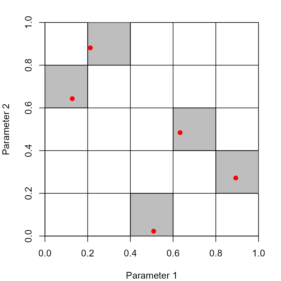
A <- randomLHS(5, 4) 
A
#>           [,1]       [,2]      [,3]      [,4]
#> [1,] 0.6328827 0.48424369 0.1678234 0.1974741
#> [2,] 0.2124960 0.88111537 0.6069217 0.4771109
#> [3,] 0.1277885 0.64327868 0.3612360 0.9862456
#> [4,] 0.8935830 0.27182878 0.4335808 0.6052341
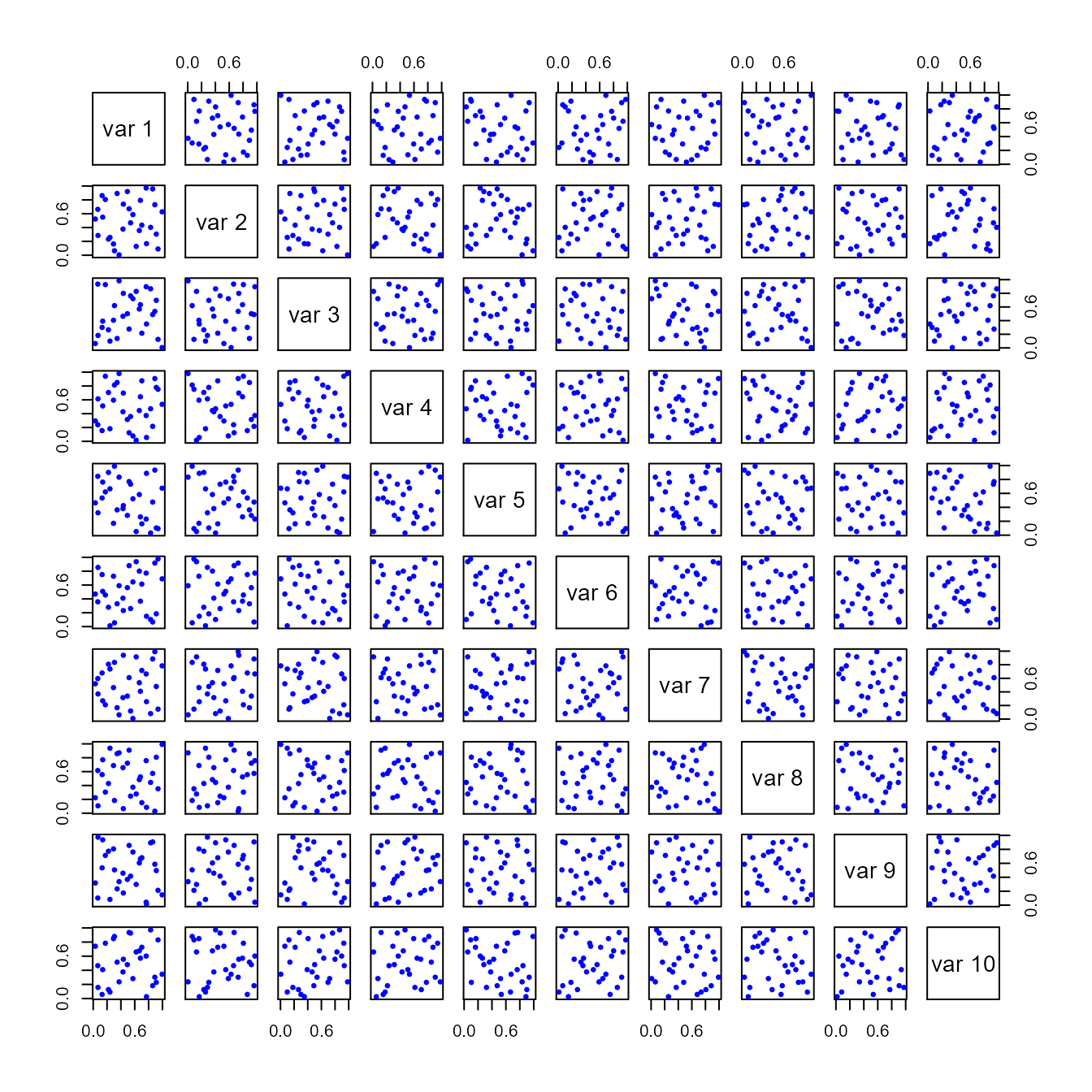
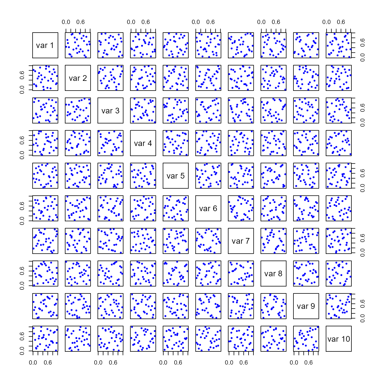
#> [5,] 0.5089423 0.02269382 0.8796676 0.2036678

In general, the LHS is uniform on the margins until transformed (Figure 1):

Figure 1. Two dimensions of a Uniform random LHS with 5 samples

It is common to transform the margins of the design (the columns) into other distributions (Figure 2)

B <- matrix(nrow = nrow(A), ncol = ncol(A))
B[,1] <- qnorm(A[,1], mean = 0, sd = 1)
B[,2] <- qlnorm(A[,2], meanlog = 0.5, sdlog = 1)
B[,3] <- A[,3]
B[,4] <- qunif(A[,4], min = 7, max = 10)
B
#>             [,1]      [,2]      [,3]     [,4]
#> [1,]  0.33949794 1.5848575 0.1678234 7.592422
#> [2,] -0.79779049 5.3686737 0.6069217 8.431333
#> [3,] -1.13690757 2.3803237 0.3612360 9.958737
#> [4,]  1.24581019 0.8982639 0.4335808 8.815702
#> [5,]  0.02241694 0.2228973 0.8796676 7.611003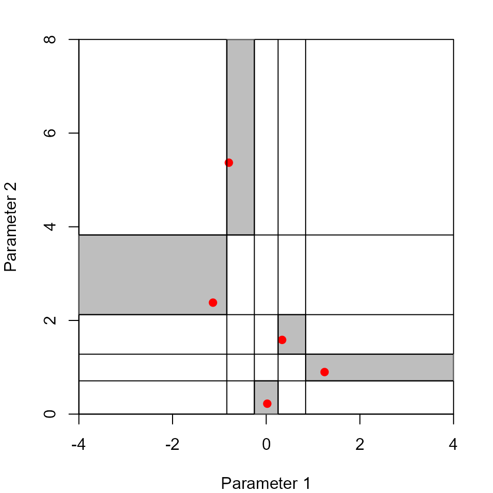

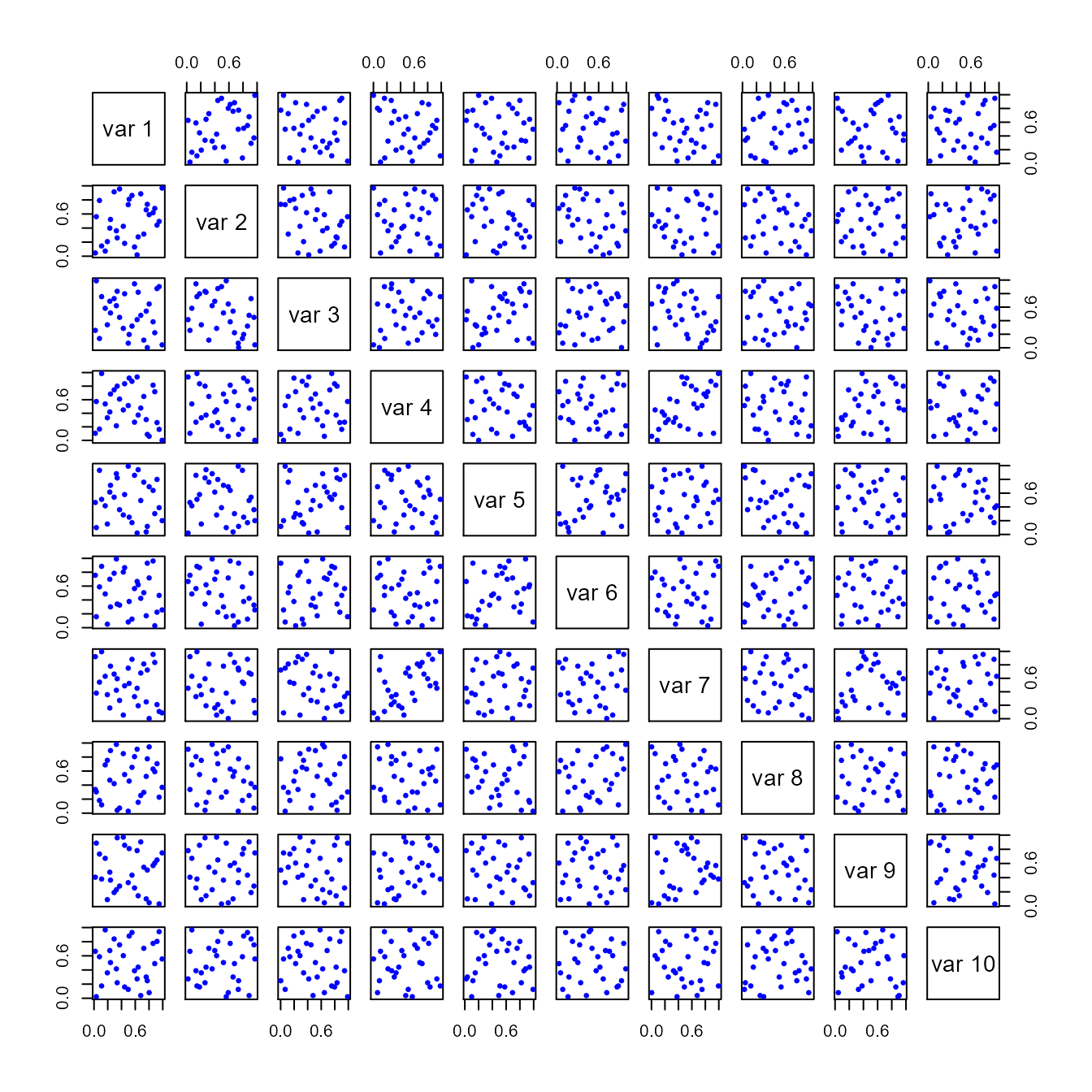
Figure 2. Two dimensions of a transformed random LHS with 5 samples

Optimizing the Design

The LHS can be optimized using a number of methods in the lhs package. Each method attempts to improve on the random design by ensuring that the selected points are as uncorrelated and space filling as possible. Table 1 shows some results. Figure 3, Figure 4, and Figure 5 show corresponding plots.

set.seed(101)
A <- randomLHS(30, 10)
A1 <- optimumLHS(30, 10, maxSweeps = 4, eps = 0.01)
A2 <- maximinLHS(30, 10, dup = 5)
A3 <- improvedLHS(30, 10, dup = 5)
A4 <- geneticLHS(30, 10, pop = 1000, gen = 8, pMut = 0.1, criterium = "S")
A5 <- geneticLHS(30, 10, pop = 1000, gen = 8, pMut = 0.1, criterium = "Maximin")

---

Table 1. Sample results and metrics of various LHS algorithms

Method	Min Distance btwn pts	Mean Distance btwn pts	Max Correlation btwn pts
randomLHS	0.6346585	1.2913235	0.5173006
optimumLHS	0.8717797	1.3001892	0.1268209
maximinLHS	0.595395	1.2835191	0.2983643
improvedLHS	0.6425673	1.2746711	0.5711527
geneticLHS (S)	0.8340751	1.3026543	0.3971539
geneticLHS (Maximin)	0.8105733	1.2933412	0.5605546

---

Figure 3. Pairwise margins of a randomLHS

---

Figure 4. Pairwise margins of a optimumLHS

---

Figure 5. Pairwise margins of a maximinLHS